Twisted Bilayer h-BN Flat Bands
1. Introduction
This tutorial calculates the band structure of the twisted hexagonal boron nitride (h-BN) bilayers created in the structure creation tutorial and reads off the width of their top set of flat valence bands, as in the following manuscript.
Manuscript
Lede Xian, Dante M. Kennes, Nicolas Tancogne-Dejean, Massimo Altarelli, and Angel Rubio, "Multiflat Bands and Strong Correlations in Twisted Bilayer Boron Nitride: Doping-Induced Correlated Insulator and Superconductor" Nano Lett. 19, 4934–4940 (2019) DOI: 10.1021/acs.nanolett.9b00986 1
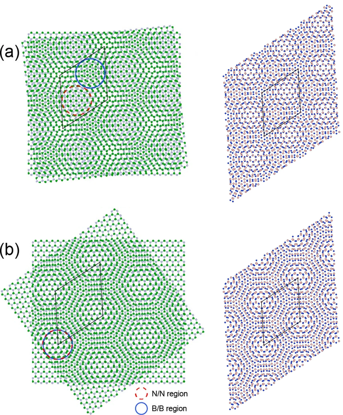
1.1. What the manuscript found
The manuscript computes the band structure of unrelaxed twisted bilayers along Γ–K–M of the moiré cell. The top set of valence bands is flat, and its width decreases from 101.4 meV at 7.34° to 1.6 meV at 2.64° (text p. 4936; Fig. 1g). This tutorial computes the 7.34° point.
2. Prerequisites
Run the
structure creation tutorial
first. Its notebook saves each bilayer and the monolayer into the uploads folder under a name such as
h-BN bilayer 7.34deg alpha d3.23, and this notebook loads them back by exactly those names.
3. What is calculated
One job per material runs the Standata "Band Structure" workflow (band_structure.json) on a
structure saved by the structure notebook. It chains pw_scf, the self-consistent run on the material's k-grid, and
pw_bands, the bands along Γ–K–M of its cell.
| structure | twist | interlayer distance | atoms |
|---|---|---|---|
h-BN bilayer 7.34deg alpha d3.23 |
60° + 7.34° (α) | 3.23 Å | 244 |
h-BN bilayer 7.34deg beta d3.23 |
7.34° (β) | 3.23 Å | 244 |
h-BN monolayer |
— | — | 2 |
The simulation notebook computes the monolayer and α by default; β and the smaller angles are
commented entries in MATERIALS.
3.1. The structure is not relaxed
The manuscript's band widths are computed with flat layers 3.23 Å apart (p. 4935–4936). The structure notebook builds the bilayers the same way, and the workflow has no relaxation step.
3.2. Which configuration the twist angle gives
Configurations α and β share one moiré cell and their twist angles differ by 60° (p. 4935). Their
unrelaxed band structures are almost identical, and the manuscript does not say which one Fig. 1g
uses (p. 4936). With the h-BN from Standata, an angle of 60 + 7.34 in the structure notebook
gives α, and 7.34 gives β.
4. Calculation parameters
The manuscript used VASP with the local density approximation (LDA) and projector augmented-wave (PAW) pseudopotentials (Supporting Information, p. 2):
| this tutorial | manuscript | |
|---|---|---|
| Code | Quantum ESPRESSO | VASP |
| Functional | LDA (pz) |
LDA |
| Pseudopotentials | ultrasoft (GBRV) | PAW |
| Cutoff | 40 Ry wavefunction, 200 Ry density | 400 eV |
| Self-consistent k-points | Γ (bilayers), 12×12×1 (monolayer) | Γ (bilayers), not stated (monolayer) |
| Band path | Γ–K–M, 7 points (bilayers), 61 points (monolayer) | Γ–K–M, number of points not stated |
| Lattice constant | 2.509 Å (Standata) | 2.512 Å |
| Interlayer distance | 3.23 Å | 3.23 Å |
| Vacuum | 20 Å above the top layer | not stated |
| Spin polarization | off | not stated |
| Geometry | not relaxed | not relaxed |
Cell 1.3 sets the DFT parameters:
1 2 3 4 5 6 7 8 9 10 11 12 | |
4.1. K-point sampling
KPATH and KPATH_MONOLAYER, in cell 1.2, list the vertices of a path and the number of steps from
each to the next; the steps values set how many points the bands are computed at. Each entry of
MATERIALS names its path under "kpath".
4.2. The band structure path belongs to the moiré cell
The path is Γ–K–M of the moiré cell, as in the manuscript's Fig. 1f and Supporting Information
Fig. S2. The manuscript gives the width of "the top of the valence bands (the first set of flat
bands)" without saying where in the Brillouin zone it is taken (p. 4936). Here it is the spread of
the top valence flat set over the points of KPATH, vertices included. The set starts at the
highest occupied band and takes in each band below whose maximum reaches the set's minimum; its
separation is the distance from the set's minimum down to the maximum of the next band.
5. Step-by-step instructions
5.1. Create the structures
Run the
structure creation notebook.
Its default parameters build the 7.34° α and β bilayers and save them as
h-BN bilayer 7.34deg alpha d3.23 and h-BN bilayer 7.34deg beta d3.23.
5.2. Open the simulation notebook
1 | |
5.3. Select the materials
Cell 1.2 holds the band paths, the materials with the k-grid, path and manuscript value of each, the workflow and the compute settings:
1 2 3 4 5 6 7 8 9 10 11 12 13 14 15 16 17 18 19 20 21 22 23 24 25 26 27 28 29 30 31 32 33 34 35 36 37 38 39 40 41 42 43 44 45 46 47 48 | |
Each name in MATERIALS must match a name the structure notebook saved; one job is created per
entry. Set ORGANIZATION_NAME to the account's organization.
5.4. Run the notebook
Select Run > Run All. The notebook will authenticate with the platform, load and save the materials, submit the jobs one after another and wait for them. Section 7 reads the band structures, the flat-band widths and the separations of the bilayers and the band gap of the monolayer, and section 8 prints them beside the manuscript's values.
6. Expected results
6.1. Flat-band width and band gap
For each bilayer the last cell prints the number of bands in the top valence flat set and its width along Γ–K–M beside the manuscript's value, and the separation of the set from the bands below; for the monolayer, its band gap along Γ–K–M beside the manuscript's. For the defaults:
| quantity | this tutorial | manuscript |
|---|---|---|
h-BN bilayer 7.34deg alpha d3.23: width of the top valence flat set (2 bands), along Γ–K–M |
101.3 meV | 101.4 meV (text p. 4936; Fig. 1g) |
h-BN bilayer 7.34deg alpha d3.23: separation from the bands below |
57.6 meV | not given at 7.34° |
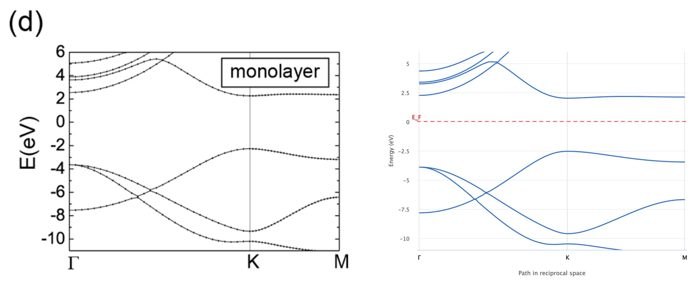
h-BN monolayer: band gap along Γ–K–M |
4.56 eV | 4.7 eV (Supporting Information, p. 10) |
6.2. Band structure of the monolayer
The manuscript's Fig. 1d beside the monolayer job's band structure as the platform plots it:
7. Troubleshooting
7.1. Material not found
ValueError: No material named … means the structure notebook has not been run, or a name in
MATERIALS differs from the names it saved. Run the
structure tutorial first.
8. Interactive JupyterLite notebook
The notebook below calculates the band structure and prints the comparison. Select Run > Run All Cells.
9. References
-
Lede Xian, Dante M. Kennes, Nicolas Tancogne-Dejean, Massimo Altarelli, and Angel Rubio. Multiflat bands and strong correlations in twisted bilayer boron nitride: doping-induced correlated insulator and superconductor. Nano Lett., 19(8):4934–4940, 2019. URL: https://doi.org/10.1021/acs.nanolett.9b00986. ↩