Gr/Ni(111) Registry and Work of Adhesion¶

1. Introduction¶

This tutorial reproduces the structure and energetics of graphene on Ni(111) — which registry the film adopts, how far it sits above the surface, and the work of adhesion of each arrangement — using the interface created in the structure creation tutorial.

Manuscript

Arjun Dahal, Matthias Batzill, "Graphene-nickel interfaces: a review" Nanoscale, 6(5), 2548 (2014) DOI: 10.1039/c3nr05279f ¹

Its computed values are from Jayeeta Lahiri et al., "Graphene growth and stability at nickel surfaces", New J. Phys. 13, 025001 (2011) DOI: 10.1088/1367-2630/13/2/025001 ²

1.1. What is being reproduced¶

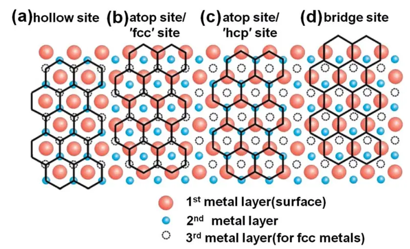
The review's computed values are from Lahiri et al. ² (New J. Phys. 13, 025001 (2011), open access), whose Table 1 is the quantitative target here:

interface	work of adhesion (J/m²)	separation (Å)
fcc (atop + fcc hollow)	0.81	2.16
hcp (atop + hcp hollow)	0.77	2.17
hollow (fcc + hcp hollows)	0.31	3.26

The bridge registry (Fig. 1d of the review) is not quantified in either paper and is computed as an extra point beyond the published set.

The four registries of graphene on a close-packed metal surface

2. Prerequisites¶

Run the structure creation tutorial first. Its notebook builds the Gr/Ni(111) interface and saves it into the uploads folder as Graphene_Nickel_interface; the simulation notebook loads it back by exactly that name and stops if it is missing. The reduced cell is the 1×1 match: 2 carbon and 4 nickel atoms.

3. Workflow overview¶

Two tiers, both relaxed:

Fast tier (MACE-MP) — each registry is placed on the substrate's own measured surface sites, bracketed by a rigid separation scan, then relaxed with atomic positions free along z only and the bottom substrate layers fixed.
Precise tier (LDA on the platform) — one fixed-cell relaxation per selected registry, starting from the MACE-relaxed geometry, at the paper's LDA functional.

Both tiers also relax the same-cell references the work of adhesion needs — a bare Ni slab and a free-standing graphene layer — under the same constraint. The work of adhesion is:

W = [E(slab) + E(graphene) − E(interface)] / A

where A is the interface area.

4. Calculation parameters¶

The published method is LDA, spin-polarized, with geometry relaxation in which the bottom two of five substrate layers are held fixed. This tutorial's fast tier holds the bottom two layers fixed; the platform tier relaxes every atom.

	fast tier	precise tier	Lahiri et al.
Method	MACE-MP-0 (large, float64) + D3	LDA (`pz`), GBRV ultrasoft	LDA, all-electron LCAO (DMol)
Spin	via training data	collinear, moment started at 0.7 μB on Ni; graphene reference unpolarized	spin-polarized (bulk Ni: 0.56 μB)
Relaxation	BFGS, z-only, bottom 2 Ni layers fixed	fixed-cell relaxation (`pw_relax`, `calculation = 'relax'`)	bottom 2 of 5 Ni layers fixed
Cutoffs	—	40 / 200 Ry (GBRV's published pair)	all-electron
k-grid	—	12×12×1 (multiple of 3, so K is on the mesh)	converged, not stated
Smearing	—	Marzari-Vanderbilt cold, `degauss = 0.01` Ry	not stated
Dispersion	D3	none — matching the paper	none

Divergences from the published method:

4 Ni layers, not 5.
20 Å of vacuum, not 90.
Plane-wave pseudopotentials, not all-electron LCAO.
The platform tier relaxes every atom, where the paper held the bottom two layers fixed.

5. Step-by-step instructions¶

5.1. Open the notebook¶

other/materials_designer/specific_examples/optimization_interface_film_xy_position_graphene_nickel_SIMULATION.ipynb

5.2. Configure parameters¶

The parameters cell sets the material and workflow parameters:

# Material parameters
FOLDER = "./uploads"
BASE_MATERIAL_NAME = "Graphene_Nickel_interface"  # created by the companion structure notebook

# Workflow parameters
WORKFLOW_SEARCH_TERM = "fixed_cell_relaxation.json"
APPLICATION_NAME = "espresso"
MY_WORKFLOW_NAME = "Fixed-cell Relaxation (Gr/Ni registry)"

5.3. Set DFT parameters¶

The same cell sets the method the precise tier submits:

# Method parameters — the published setup (Lahiri et al., section 2.2) where the platform can
# express it: LDA, spin-polarized, relaxed, no dispersion correction.
PSEUDOPOTENTIAL_TYPE = "us"
FUNCTIONAL = "pz"
MODEL_SUBTYPE = "lda"
ECUTWFC = 40   # GBRV's published pair
ECUTRHO = 200
SCF_KGRID = [12, 12, 1]  # multiple of 3 keeps K on the mesh; dense for a metal
STARTING_MAGNETIZATION = {"Ni": 0.7}  # near the bulk moment

# SCF settings for a spin-polarized metal slab
SMEARING = "mv"
DEGAUSS = 0.01  # Ry
ADDITIONAL_PARAMETERS = {
    "electrons": {
        "mixing_mode": "local-TF",
        "mixing_beta": 0.2,
        "electron_maxstep": 200,
    },
}

5.4. Run the fast tier¶

Run > Run All Cells. Sections 2–4 need no platform account: they load the interface, place each registry, relax it with MACE, and print the comparison against Lahiri Table 1.

5.5. Run the precise tier¶

Section 5 selects which registries submit to the platform. DFT_REGISTRY_NAMES ships with one registry active and three commented out:

DFT_REGISTRY_NAMES = [
    "atop_fcc",
    # "atop_hcp",
    # "hollow",
    # "bridge",
]

Running the rest of section 5 authenticates and submits a relaxation + total-energy job for each name in the list, plus the two reference jobs. Leaving DFT_REGISTRY_NAMES empty skips the platform tier; the automated test does exactly that, because relaxation jobs outlast what a browser test may wait for.

5.6. Read the final table¶

The final cell prints the computed values beside the published ones: work of adhesion, separation and buckling for each registry, in paper / MACE / DFT columns, with — wherever a tier did not run or the paper gives no value.

6. Expected results¶

The fast tier prints these values for the four registries, beside Lahiri et al.'s Table 1:

registry	MACE W_adh (J/m²)	MACE separation (Å)	MACE buckling (Å)	paper W_adh (J/m²)	paper separation (Å)
atop_fcc	0.17	1.98	−0.006	0.81	2.16
atop_hcp	0.14	1.98	−0.004	0.77	2.17
hollow	0.30	4.08	—	0.31	3.26
bridge	0.05	1.97	—	—	—

A single precise-tier job, run on the platform for atop_fcc, gave a work of adhesion of 1.01 J/m², a separation of 2.02 Å, and a buckling of +0.013 Å with the atop carbon outward; the registry was preserved.

7. Customization options¶

7.1. Submit more registries¶

Uncomment additional entries in DFT_REGISTRY_NAMES to submit more precise-tier jobs:

DFT_REGISTRY_NAMES = [
    "atop_fcc",
    "atop_hcp",
    "hollow",
    "bridge",
]

7.2. Adjust computational resources¶

Modify the compute parameters in the parameters cell:

CLUSTER_NAME = None  # or a specific cluster name
QUEUE_NAME = QueueName.OF
PPN = 40
TIME_LIMIT = "04:00:00"

7.3. Swap the MLFF model¶

Change the fast-tier force field in the parameters cell:

MACE_MODEL_FAMILY = "MACE-MP-0"
MACE_MODEL = "large"
MACE_DEFAULT_DTYPE = "float64"

8. Interactive JupyterLite notebook¶

The notebook below runs the fast tier and, when registries are selected, the platform tier. Select Run > Run All Cells.

9. References¶

Arjun Dahal and Matthias Batzill. Graphene–nickel interfaces: a review. Nanoscale, 6:2548–2562, 2014. URL: https://doi.org/10.1039/C3NR05279F. ↩
Jayeeta Lahiri, Travis S. Miller, Andrew J. Ross, Lyudmyla Adamska, Ivan I. Oleynik, and Matthias Batzill. Graphene growth and stability at nickel surfaces. New Journal of Physics, 13:025001, 2011. URL: https://doi.org/10.1088/1367-2630/13/2/025001, doi:10.1088/1367-2630/13/2/025001. ↩↩