GaAs/AlAs (110) Strained Superlattice

1. Introduction

This tutorial creates the GaAs/AlAs (110) superlattice of the following manuscript, together with the two strained bulk cells its valence band offset is computed from.

Manuscript

Yoyo Hinuma, Andreas Grüneis, Georg Kresse and Fumiyasu Oba, "Band alignment of semiconductors from density-functional theory and many-body perturbation theory", Physical Review B 90, 155405 (2014). DOI: 10.1103/PhysRevB.90.155405. ¹

The superlattice stacks GaAs and AlAs along [110] without vacuum, so it has two identical interfaces. Both materials are strained to the mean of their two lattice constants and stay cubic as built; the manuscript relaxed the out-of-plane lattice. The manuscript uses 11 atomic layers of each material; the slab builder counts (110) layers in pairs of atomic planes, so the notebook builds 12 planes of each (6 layers), 48 atoms in total.

The offset needs, besides the superlattice, separate bulk cells of GaAs and of AlAs strained as in the superlattice, so the notebook saves all three.

2. Open the notebook

2.1. Load the base materials

The notebook loads GaAs (mp-2534) and AlAs (mp-2172) from Standata, so no input material needs to be selected.

2.2. Launch JupyterLite session

Select the "Advanced > JupyterLite Transformation" menu item to launch the JupyterLite environment, or use the notebook embedded in Section 6.

2.3. Open interface_3d_3d_gallium_arsenide_aluminum_arsenide.ipynb notebook

Find and open interface_3d_3d_gallium_arsenide_aluminum_arsenide.ipynb in the specific_examples folder.

3. Configure and create the structure

3.1. Set parameters

Cell 1.1 of the notebook sets the materials, the slab thickness, and the names of the saved materials:

SUBSTRATE_NAME = "mp-2534"  # GaAs, Standata
FILM_NAME = "mp-2172"  # AlAs, Standata
MILLER_INDICES = (1, 1, 0)
NUMBER_OF_LAYERS = 6  # conventional (110) layers, two atomic planes each

SUPERLATTICE_NAME = "GaAs/AlAs (110) superlattice 12+12"
SUBSTRATE_BULK_NAME = "GaAs (110) bulk strained"
FILM_BULK_NAME = "AlAs (110) bulk strained"

3.2. Run the notebook

Execute the notebook by selecting "Run" > "Run All Cells" from the JupyterLite menu.

3.3. Follow the construction

The notebook builds the superlattice in four steps:

1. Each bulk is converted to its conventional cubic cell and strained to the mean lattice constant, which the notebook prints together with the misfit. The strain comes first: the interface builder re-creates its slabs from the bulk, so a strain applied to a slab would be lost.
2. A slab of NUMBER_OF_LAYERS conventional (110) layers is cut from each strained bulk, without vacuum.
3. The slabs are joined without gap or vacuum, and the cell is reduced to the primitive cell. The periodic boundary closes the second interface.
4. One (110) layer of each strained bulk, periodic along the stacking axis, is cut as the bulk reference cell of the valence band offset. Atom labels are removed from all three materials, because labels break the Quantum ESPRESSO input.

4. Analyze the structure

Section 2.4 of the notebook prints the composition, the cell, the plane spacings along c and the number of nearest neighbors of each atom for the three materials; it raises an error if an atom is not four-coordinated, as every atom is in the zincblende structure:

GaAs/AlAs (110) superlattice 12+12: {'Al': 12, 'Ga': 12, 'As': 24}, 48 atoms, cell 4.0397 x 5.7130 x 48.4763 Å
  plane spacings along c: [2.0198, 2.0199] Å
  coordination numbers: {4: 48}
GaAs (110) bulk strained: {'Ga': 4, 'As': 4}, 8 atoms, cell 5.7130 x 8.0794 x 4.0397 Å
  plane spacings along c: [2.0198, 2.0199] Å
  coordination numbers: {4: 8}
AlAs (110) bulk strained: {'Al': 4, 'As': 4}, 8 atoms, cell 5.7130 x 8.0794 x 4.0397 Å
  plane spacings along c: [2.0198, 2.0199] Å
  coordination numbers: {4: 8}

The planes are evenly spaced across both interfaces. The picture below is drawn from the notebook's superlattice, seen along a with c horizontal; the dotted box outlines the cell along c and three cells along b:

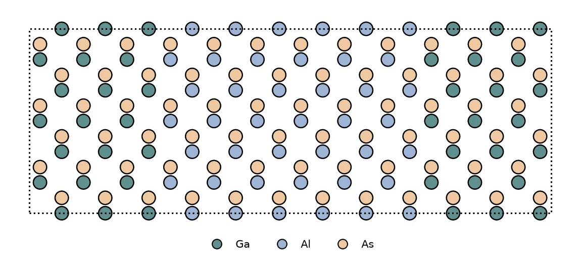
The GaAs block appears split between the bottom and the top of the cell. The reduction to the primitive cell places the cell origin on a symmetry plane of the superlattice, the centre of the GaAs block; across the periodic boundary it is one continuous block of 12 planes. Only the appearance changes, not the structure.

5. Save the structure

Section 4 of the notebook sends the three materials to the environment. In JupyterLite they are passed to Materials Designer, where they can be saved on the platform; in a local Jupyter session they are written to the uploads folder.

6. Interactive JupyterLite notebook

The following JupyterLite notebook creates the superlattice and the two bulk cells. Select "Run" > "Run All Cells".

⛶ Full Screen

7. References

---

1. Yoyo Hinuma, Andreas Grüneis, Georg Kresse, and Fumiyasu Oba. Band alignment of semiconductors from density-functional theory and many-body perturbation theory. Physical Review B, 90:155405, 2014. URL: https://link.aps.org/doi/10.1103/PhysRevB.90.155405. ↩